MovieLens-25m Experiments (Part 1): Matrix Factorization
28 Oct 2022Matrix factorization is one of the most recognized ways to generate recommendations. In this post, we explore matrix factorization for a specific dataset. We will start with a simple model and add variations to it as we go along.
Let’s consider the movielens-25m dataset. Movielens datasets are widely used for recommendation system research. The Movielens-25m dataset is fairly straightforward. It contains 25 million ratings by some >160k users. A rating can range from 0.5 to 5.0 in increments of 0.5: 0.5, 1.0, 1.5, 2.0, 2.5, 3.0, 3.5, 4.0, 4.5, 5.0. It’s a 10-class classification problem. If you randomly choose a rating, you would be correct 10% of the time. We want to do better than random.
We will model this rating prediction problem as a regression problem. The 10 classes are not completely independent. There is a nice sliding scale from 0.5 to 5.0, which makes regression a better choice. However, we will stick with test accuracy to compare our models (instead of MSE or other regression metrics). Regression output is mapped to 10 classes by scaling the output from 0.25 to 5.25 and finding the nearest rating.
Matrix Factorization
Let’s take a quick recap of matrix factorization for recommendations. The end goal is to learn \(d\)-dimensional user embeddings and \(d\)-dimensional movie embeddings. Let’s say we have \(n\) users and \(m\) movies. We want to learn \(U_{n \times d}\) (n rows of \(d\)-dimensional vectors) and \(M_{m \times d}\) (m rows of \(d\)-dimensional vectors) matrices. Let’s denote our rating matrix as \(R_{n \times m}\).
\[U_{n \times d} \cdot \left(M_{m \times d}\right)^\top = R_{n \times m}\]Our goal is to learn \(U_{n \times d}\) and \(M_{m \times d}\) such that their matrix multiplication approximates \(R_{n \times m}\).
\(R_{n \times m}\) matrix is sparse, because not every user is going to rate every movie. Most users will rate only a very small subset of movies. We will ignore the missing ratings completely and only learn from the ratings we do have. We optimize the mean squared error loss for the observed entries. In its simplest form, the loss looks like the following:
\[\frac{1}{n} \sum_i{(r_i - u_i \cdot m_i)}^2\]\(r_i\) is the observed rating, \(u_i\) is the \(d\)-dimensional user embedding vector, and \(m_i\) is the \(d\)-dimensional movie embedding vector. \(u_i \cdot m_i\) is the dot product between the user and movie vectors. It’s often a good idea to add the L2 norm to the loss function for regularization:
\[\frac{1}{n} \sum_i{(r_i - u_i \cdot m_i)}^2 + \alpha * ||params||\]\(\alpha\) is the regularization parameter above, and it’s multiplied by the L2 norm of all parameters including user and movie embeddings.
User and Movie Bias
Let’s consider a variant of the matrix factorization described above. Let’s say we have a user Bob in our list of users. Bob never rates any movie above 2.0 no matter what. By adding user bias to the mix, our model can better adapt to users like Bob. Similarly, movie bias achieves the same purpose to adapt to different movies:
\[U_{n \times d} \cdot \left(M_{m \times d}\right)^\top + B^U_{n \times 1} \cdot J_{1 \times m} + J_{n \times 1} \cdot \left(B^M_{m \times 1}\right)^\top = R_{n \times m}\]The first term in the above equation is the same as our matrix multiplication above. \(B^U_{n \times 1}\) is the user bias matrix, where each row represents a 1-dimensional bias for a user. Similarly, \(B^M_{m \times 1}\) is the movie bias matrix, where each row represents a 1-dimensional bias for a movie. Matrix \(J\) is a matrix of ones used to map \(B^U\) and \(B^M\) matrices to \(n \times m\) dimension.
In our code, we won’t need matrix \(J\) because we are only using the user-movie pairs with a rating for training purposes. So, we can simply add the 1-dimensional movie bias and the 1-dimensional user bias to predict the rating.
Side Features
Let’s consider another variant of the matrix factorization described above. Let’s say we also know the genre of each movie. How do we use this new information to improve our prediction? We can learn genre embeddings as well and make that a part of our matrix multiplication equation:
\[U_{n \times d} \cdot \left(M_{m \times d}\right)^\top + U_{n \times d} \cdot \left(G_{p \times d}\right)^\top = R_{n \times m}\]\(G_{p \times d}\) is the embedding matrix for genres, where each row is a \(d\)-dimensional genre embedding. It has \(p\) rows, each row representing a genre.
Model Training
I am using pytorch to train my models. The code is in this repository - github.com/hardikp/movielens. Each code file is self-contained to make it easier to follow & replicate.
Model training results are the most interesting to me since they give a sense of what works in practice and what doesn’t work. That’s covered in the next section.
Results and Discussion
Our matrix factorization model learns \(d\)-dimensional embedding vectors for users as well as movies. The choice of \(d\) dimension makes a difference in how accurately you can predict test labels.
Embedding Size
There are a few ways to look at the test accuracy variations as we increase the embedding size. This is the first one:
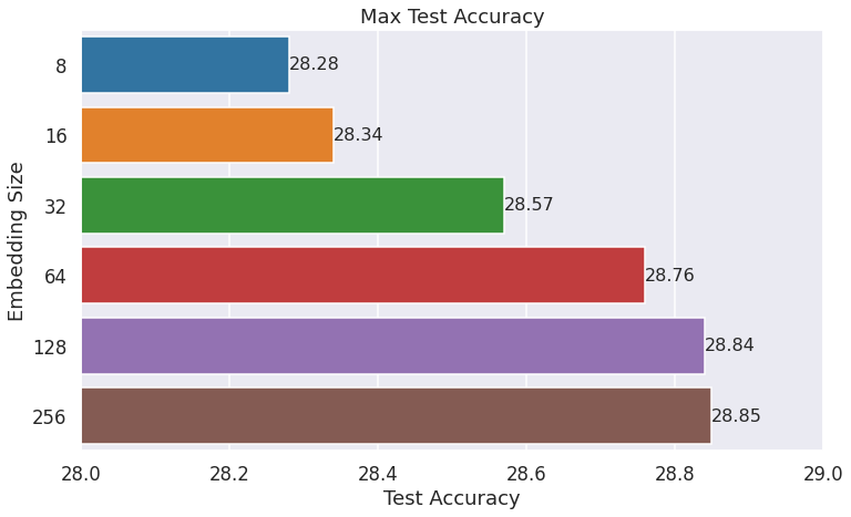
The above bar plot shows the max test accuracy observed for different embedding sizes throughout model training. Each model is trained over 50 epochs, with a learning rate of 0.001 and batch_size of 512. Test accuracy increases as we increase the embedding vector size before plateauing after 128 embedding size.
However, increasing embedding size increases the difference between train accuracy and test accuracy. If train accuracy is considerably high but test accuracy is relatively low, it’s a sign that there is overfitting and the model may not generalize well to new rating data. The following plot shows the difference between train accuracy and test accuracy for different embedding sizes:
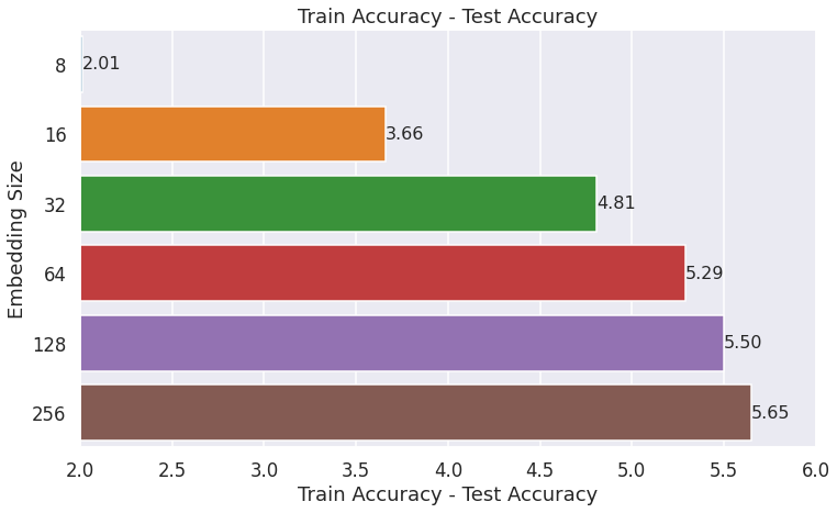
The above plot shows that the risk of overfitting increases as we increase the embedding vector size. One common way to address the train/test drift seen above is to add regularization. We discuss the results of adding L2 regularization later in this post.
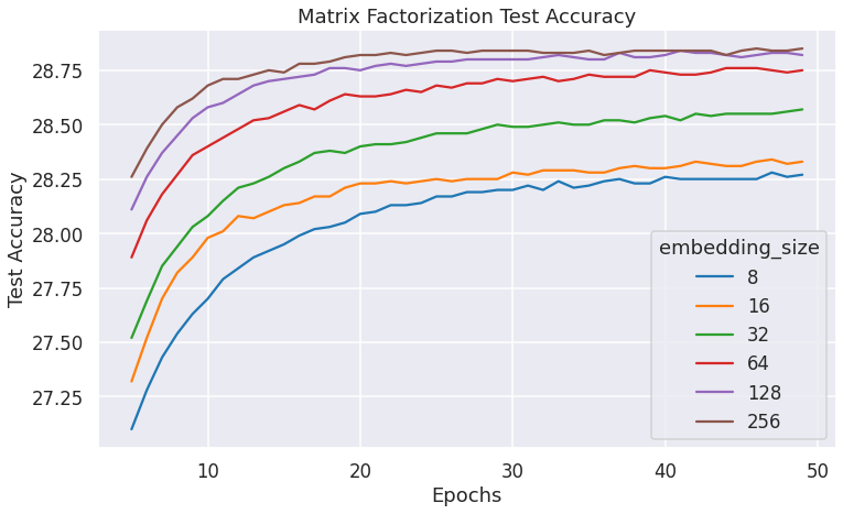
On a separate note, the following plot shows how quickly various models improve test accuracy over epochs:
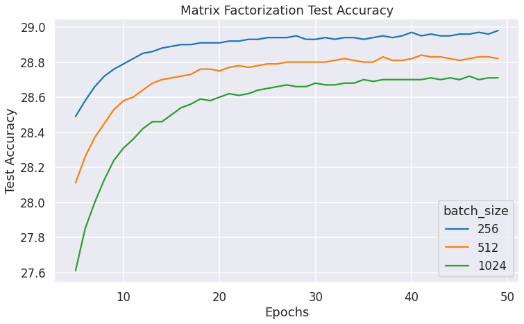
Batch Size
Smaller batch sizes help learn the model weights faster. But, it also takes longer for them to finish training. The whole purpose of batching inputs is to utilize the SIMD nature of GPUs to speed up training. Unsurprisingly, we can see that the test accuracy is better with smaller batch_sizes:
Learning Rate
The learning rate is another important hyperparameter. A high learning rate helps get the model to a good loss area quickly. But, the learning can become unstable after the initial success. On the other end, a low learning rate makes the model training slow. Ideally, we should utilize an adaptive learning rate schedule where we start with a high learning rate and slowly decrease the learning rate as training progresses. The following graph shows model training with various fixed learning rates.
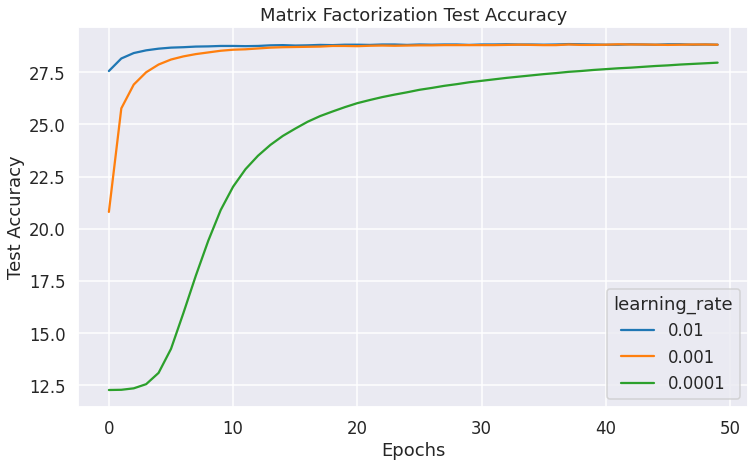
It shows that the low learning rate model takes a long time before the test accuracy improves considerably. On the other hand, the high learning rate model quickly reaches a good loss area and stays there for the rest of the epochs.
Ideally, it would be best to start with a high learning rate and then slowly decrease it. But, I didn’t try that here. I suspect the benefits of adaptive learning rates are higher for more complex models, but it should certainly help in our case as well given the above graph.
L2 Regularization
We saw that higher embedding dimension models had high differences between train accuracy and test accuracy. One way to reduce it is to add regularization. The following graph shows that more weight for L2 regularization leads to better coherency between the train set and the test set.
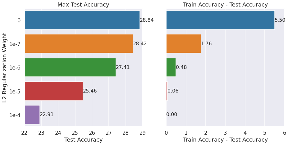
However, it comes at the cost of reduced max test accuracy as seen above. So, we need to find a good balance in practice.
L2 Regularization vs Dropout
Dropout is a popular way to regularize neural networks. It’s usually not used for embedding layers, even though that’s how we will apply it here. We will mask out some parts of each embedding depending on the dropout probability. The following graph shows that the 0.15 dropout helps increase the max accuracy while reducing the train-test drift compared to no regularization at all. However, 0.25 dropout is too much, leading to reduced max accuracy.
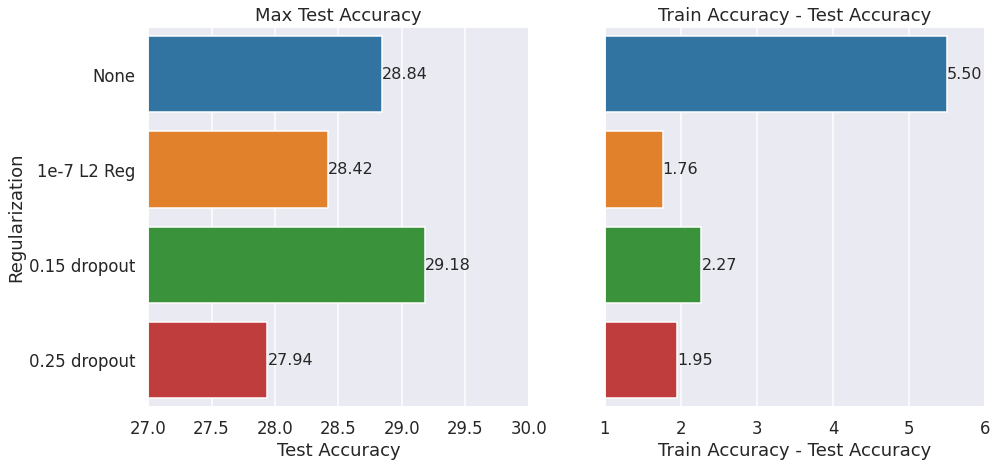
Dropout seems surprisingly effective at reducing train-test drift. My mental model was that dropout is essential for neural networks. But, L1 or L2 regularization is more effective for classic linear regression models. I didn’t know what to expect for matrix factorization models. Turns out that both L2 regularization and dropout are similarly effective.
User & Movie Biases
We discussed the idea of adding movie & user biases earlier in this post. The following bar graph shows that test accuracies increase if we add movie and user biases. We compare 2 models:
- Base (no biases) model with 1e-7 L2 regularization weight
- Movie + User biases with 1e-6 L2 regularization weight
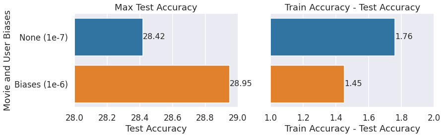
We are using only models with L2 regularization for comparison here. That’s because adding movie & user biases makes the diverging train & test accuracy problem worse. Notice that we need to increase the L2 regularization weight since we made the model more complex. But, the added movie & user biases end up increasing the test accuracy even while decreasing the train/test drift with the appropriate regularization factor.
User Bias vs Movie Bias
We added both the user bias and the movie bias above. It’s interesting to note which of the two is more important. From the following graph, it looks like movie bias is more important.
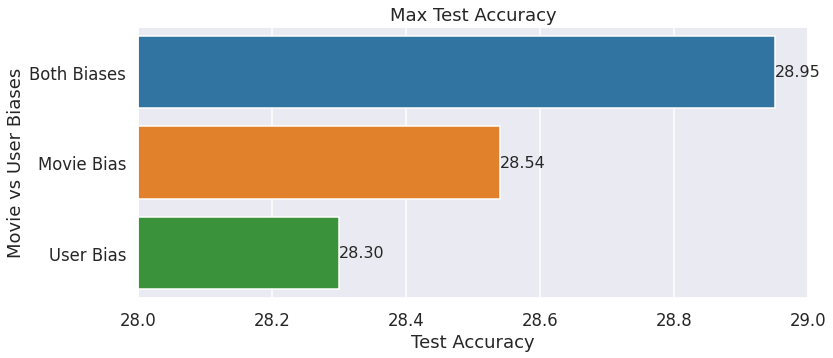
The same 1e-6 L2 regularization weight was used for training.
Side Features
We mentioned adding side features earlier in this post. The following bar graph shows that test accuracy increases if we add side features. We compare 2 models:
- Base: No side features + movie & user biases + 1e-6 L2 regularization weight
- Side Features: genre & year movie features + movie & user biases + 1e-6 L2 regularization weight
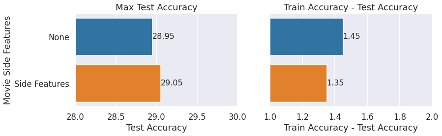
Similar to the bias case above, adding side features reduces the train_accuracy - test_accuracy diff while increasing test accuracy.
Conclusion
My aim here was to show different factors that contribute to the effectiveness of matrix factorization for recommendation use cases. I covered some variations that highlight those factors.
I hope to cover other recommendation models in a future post.
Change Log
- 2022-10-18: Original post.
- 2022-10-30: Added L2 regularization vs dropout comparison as well as movie bias vs user bias comparison. Also, some graphs and graph labels are updated/fixed.