Stock Movement Prediction from Tweets and Historical Prices (Paper Summary)
24 May 2018This paper suggests a way of using both historical prices and text data together for financial time series prediction. They call it Stocknet. There seem to be 2 major contributions here: (a) Encoding both market data and text data together, (b) VAE (Variational AutoEncoder) inspired generative model.
TLDR
RNN-based variational autoencoder along with attention is used to predict whether the stock price will go up or down.
Dataset
- 88 stocks
- From 2014-01-01 to 2016-01-01. Training data range: 2014-01-01 to 2015-08-01 (20,339 samples). Validation: 2015-08-01 to 2015-10-01 (2555 datapoints). Testing: 2015-10-01 to 2016-01-01 (3720 datapoints).
- price_change <= -0.5% is assigned 0 label. price_change > 0.55% is assigned 1 label. The ones in between these 2 thresholds are ignored.
Model
There are 3 main components here:
- Market Information Encoder (MIE) - Encodes tweets and prices to X.
- Variational Movement Decoder (VMD) - Infers Z with X, y and decodes stock movements y from X, Z.
- Attentive Temporal Auxiliary (ATA) - Integrates temporal loss through an attention mechanism for model training.
Market Information Encoder (MIE)
This component is relatively straightforward. Tweets for the given day are combined into the vector \(c_t\). Historical prices are normalized and stored in the vector \(p_t\). The output of this component (MIE) is the vector \(x_t = [c_t, p_t]\).
Variational Movement Decoder (VMD)
VMD uses the market information \(X\) received from the previous component and infers a latent factor \(Z\). This latent vector \(Z\) is then decoded into vector \(y_t\) using an RNN decoder with GRU cells.
Attentive Temporal Auxiliary (ATA)
Attention is applied to the outputs from the previous component. Both VAE and Attention components are combined to construct the final loss function \(F\).
\[F(\theta, \phi, X, y) = \frac{1}{N}\sum_n^Nv^{(n)}f^{(n)}\]Here, \(v^{(n)}\) is the attention weight vector and \(f^{(n)}\) is the loss function from the variational autoencoder component.
\[\begin{aligned} f = \log p_{\theta} - \lambda D_{KL}[q_{\phi} \vert\vert p_{\theta}] \end{aligned}\]\(\log p_{\theta}\) is the log-likelihood term, \(D_{KL}[q_{\phi} \vert\vert p_{\theta}]\) is the KL divergence loss and \(\lambda\) is the KL loss weight. \(\lambda\) is increased over time during training. It’s known as KL annealing trick Bowman et al., 2016.
Training and Hyperparameters
- 5-day lag window is used to construct the dataset.
- Batch size is 32. Each batch contains randomly picked data points.
- Initial learning rate of Adam - 0.001
- Dropout rate - 0.3 for the hidden layer
Metrics and Results
MCC (Matthews Correlation Coefficient) is used as a metric. MCC is defined below in terms of tp (true positives), tn (true negatives), fp (false positives) and fn (false negatives).
\[MCC = \frac{tp \times tn - fp \times fn}{\sqrt{(tp + fp)(tp + fn)(tn + fp)(tn + fn)}}\]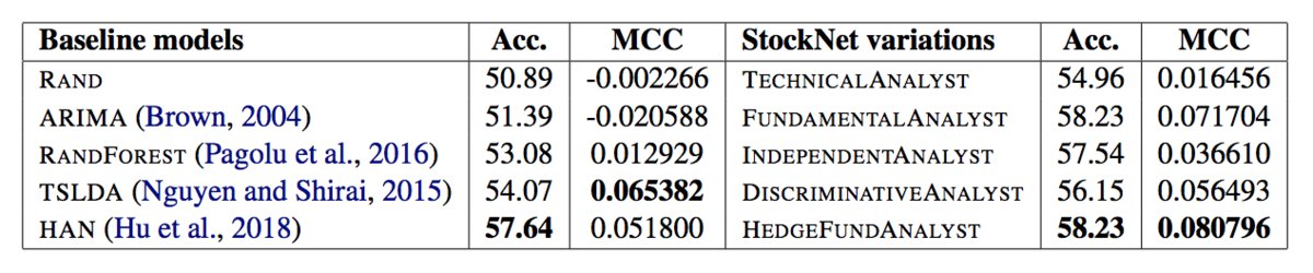
Baselines:
- RAND: Random Up or Down guess
- ARIMA
- RANDFOREST: Random Forest classifier using Word2vec text representation.
- TSLDA: Generative topic model jointly learning topics and sentiment from Nguyen and Shirai, 2015.
- HAN: Discriminative deep neural network with hierarchical attention from Hu et al., 2018.
TECHNICALANALYST, FUNDAMENTALANALYST, INDEPENDENTANALYST, DISCRIMINATIVEANALYST and HEDGEFUNDANALYST are simply different variants of their StockNet model with HEDGEFUNDANALYST being the model described above.