Machine Learning for Intraday Stock Price Prediction 1: Linear Models
03 Oct 2017This is the first of a series of posts on the task of applying machine learning for intraday stock price/return prediction. Price prediction is extremely crucial to most trading firms. People have been using various prediction techniques for many years. We will explore those techniques as well as recently popular algorithms like neural networks. In this post, we will focus on applying linear models on the features derived from market data.
Problem definition
The goal is to predict the price change (or return) of a security.
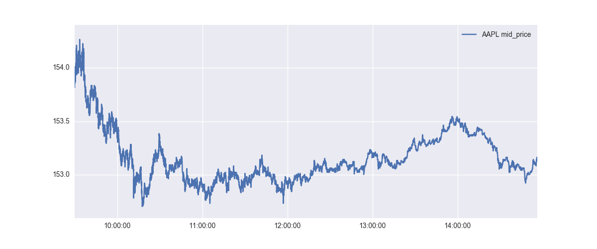
At each point in the above graph, we want to predict the prices after 1 min. Let’s look at the individual points in the above graph - there are more than 200,000 datapoints there, but we will just look at the first few to understand what it is that we want to predict.
| Timestamp (EST) | Current Price | Price after 1 min | Price Difference |
|---|---|---|---|
| 09:30:01.500000 | 153.905 | 154.03 | 0.125 |
| 09:30:01.525000 | 153.905 | 154.03 | 0.125 |
| 09:30:01.550000 | 153.905 | 154.03 | 0.125 |
| 09:30:01.575000 | 153.905 | 154.03 | 0.125 |
| 09:30:01.600000 | 153.9 | 154.03 | 0.13 |
| 09:30:01.625000 | 153.9 | 154.03 | 0.13 |
| 09:30:01.650000 | 153.905 | 154.035 | 0.13 |
| 09:30:01.675000 | 153.905 | 154.035 | 0.13 |
| 09:30:01.700000 | 153.905 | 154.035 | 0.13 |
| 09:30:01.725000 | 153.905 | 154.035 | 0.13 |
We can see that the AAPL prices are supposed to go up by $0.13 in the next 1 min. We want to build a regression algorithm to predict this price difference. Of course, it goes without saying that this is an incredibly hard problem. Even a mild success can be enormously profitable.
Please note that it’s typically better to predict returns rather than price difference because models/techniques designed to predict returns can scale across various securities relatively better. $0.13 price difference for a $154 stock is not much compared to $0.13 price difference for a $20 stock - $0.13 has a different meaning for a $20 stock. This issue doesn’t happen if you work in the return space. To convert to returns, we just divide the price difference by current price. In our AAPL example, that prediction return would come out to be 0.000843. However, we will only focus on the price difference prediction for the time being.
Data Preprocessing
Stock prices can get affected by a multitude of factors. The following are some of these factors:
- Market liquidity. Supply and demand is the most crucial factor affecting the day-to-day price change of most stocks. If Norway wealth fund decides to invest in a specific company, they will have a hard time finding liquidity - which will inevitably increase the stock price.
- News on specific stocks. Trump’s tweets have been found to affect the stock prices significantly. There have been a number of academic studies citing the effect of news/blogs/tweets on the stock prices.
- Global events can significantly affect prices. Some such recent events include US elections in Nov 2016, Brexit vote, Chinese volatility in early 2016, Russia invading Ukraine.
Effects of the above factors span different time horizons. For example, news on a specific stock would generally affect the price for the next 1-3 days. The effect of Global events can last upto a few weeks. In this post though, we will only use the features derived from the market data to predict the next 1 min price change. (We will explore news/text data effects in a separate post in future.)
Data source
- Training Period: 20170901 to 20170915 (10 days)
- Testing Period: 20170918 to 20170922 (5 days)
- 15 ETFs were selected as source securities. In other words, features derived from these 15 ETFs was used to predict the price difference. These ETFs are: SPY, BND, XLK, XLU, VNQ, IEMG, AGG, VWO, XLF, EEM, QQQ, USO, GDX, IWM, VEA
- Number of train examples: 2026106
- Number of test examples: 966630
- Mean of the price change: 0.0002
- Standard deviation of the price change: 0.0216 (Stdev helps put the Mean Absolute Error values in context)
Features
The feature set can be broadly classified into two categories: Features describing current market snapshot and Features describing recent history
- bid price, ask price
- mid price (average of bid and ask prices)
- bid size, ask size
- bid-ask spread
- Moving averages of bid price, ask price and mid price. Moving prices are computed over 1 min and 5 min intervals.
- 1 min and 5 min trends of bid price, ask price and mid price.
- volume/trades/updates over the last 1 min and 5 min intervals

We will skip the mathematical details of these features for the time being. However, please note that these features try to capture the current market conditions as well as the recent past.
Normalization
Raw values of the above features have very different scales. While the price of AAPL could range from 153 to 155 in a day, the volume over last 5 min could range from 100 to 1000000. Since most of the learning algorithms work best when the scale of the input features is similar. That’s why normalization step is crucial. I tried out few custom scaling techniques, but found that scikit-learn’s RobustScaler works quite well.
Linear Models
Let’s first try out simple linear models on this dataset.
Ordinary Least Squares Regression

Let \(x\) be the real-valued feature vector and \(y\) be the real value we want to predict. \(\theta\) are the model parameters we want to learn.
\[h(x) = \sum_{i=0}^n \theta_i x_i = \theta^Tx\]The Ordinary Least Squares Regression tries to minimize the following loss function.
\[J(\theta) = \frac{1}{2m}\sum_{i=1}^m (h(x^{(i)}) - y^{(i)})^2\]LinearRegression class from scikit-learn is used to generate the model. Unsurprisingly, the model overfits!
| InSample | OutSample | |
|---|---|---|
| MSE | 0.000242 | 43997.8 |
| MAE | 0.01184 | 151.201 |
| Original Stdev | 0.0159 | 0.0202 |
| Predicted Stdev | 0.0108 | 179.11 |
In the above table, MSE refers to Mean Squared Error and MAE refers to Mean Absolute Error. InSample refers to the training data and OutSample refers to the testing data. i.e. MAE on OutSample mean mean absolute error on the testing dataset.
Standard deviation of the predicted value has a useful information. Mean of the intraday price change is generally close to 0. This dataset has a lot of noise and not much signal. The combination of these two often makes predicting 0 for all possible \(x\) a good choice. However, the model outputing 0 is of absolutely no value - we want opinionated models that can be useful for trading or execution. Therefore, comparing the standard deviation of the predicted value \(h(x)\) with the standard deviation of \(y\) is necessary.
L2 Penalized Linear Regression
Adding a weight penalty to the error term is a simple way to regularize the model - this helps stabilize the training and the model is often better at generalization. The next experiment I did was to train a Ridge Regression model (L2 penalized linear regression) and check the out-of-sample performance.
\[J(\theta) = \frac{1}{2m}\sum_{i=1}^m (h(x^{(i)}) - y^{(i)})^2 + \alpha ||\theta||_2^2\]The following results were obtained by training a ElasticNet model with l1_ratio=0, alphas=[1e-3, 1e-4, 1e-5] and fit_intercept=False.
| InSample | OutSample | |
|---|---|---|
| MSE | 0.000219 | 0.000557 |
| MAE | 0.01101 | 0.01722 |
| Original Stdev | 0.0159 | 0.0202 |
| Predicted Stdev | 0.0050 | 0.0121 |
We can see that the out-of-sample results are much better than the LinearRegression model. Out of sample Mean Absolute Error of 0.01722 is really good in my opinion. While the standard deviation of the predicted value is a bit less, it’s still in the same range as that of \(y\).
L1 Penalized Linear Regression
Another option is to add L1 penalty to the loss function. This is also called Lasso.
\[J(\theta) = \frac{1}{2m}\sum_{i=1}^m (h(x^{(i)}) - y^{(i)})^2 + \beta ||\theta||\]The following results were obtained by training a ElasticNet model with l1_ratio=1, alphas=[1e-3, 1e-4, 1e-5] and fit_intercept=False.
| InSample | OutSample | |
|---|---|---|
| MSE | 0.000244 | 0.000412 |
| MAE | 0.01113 | 0.01313 |
| Original Stdev | 0.0159 | 0.0202 |
| Predicted Stdev | 0.0020 | 0.0018 |
Out of sample MAE is much better than that of Ridge Regression. However, the standard deviation is really low.
L1 + L2 Penalized Linear Regression
We can also add both L1 and L2 penalties to the loss function.
\[J(\theta) = \frac{1}{2m}\sum_{i=1}^m (h(x^{(i)}) - y^{(i)})^2 + \alpha ||\theta||_2^2 + \beta ||\theta||\]The following results were obtained by training a ElasticNet model with l1_ratio=0.1, alphas=[1e-3, 1e-4, 1e-5] and fit_intercept=False.
| InSample | OutSample | |
|---|---|---|
| MSE | 0.000244 | 0.000412 |
| MAE | 0.01114 | 0.01311 |
| Original Stdev | 0.0159 | 0.0202 |
| Predicted Stdev | 0.0020 | 0.0017 |
The results are similar to that of Lasso.
Other experiments on linear models
- I used all the data available for the above results, hoping that more data helps. This means all of the above models were trained on about 2 million datapoints each containing 360 features. However, in the further experiments, it was kinda clear that sampling fewer examples from 2 million points also produces the same results. Results degrade for less than 2000 examples.
- Feature selection strategies did not really add any value. In fact, the results were a bit worse.
- Dimension reduction using PCA did not change the results.
- It often helps to sample the datapoints properly. For example, selecting more datapoints involving trade (as opposed market book update) can help. Similarly, selecting datapoints from higher standard deviation periods (time intervals involving a lot more price change) helps as well.
Ensemble Models
| Algorithm | OutSample Stdev | InSample Stdev | OutSample MAE |
|---|---|---|---|
| Gradient Boosting | 0.0075 | 0.0038 | 0.01583 |
| AdaBoost | 0.0037 | 0.0058 | 0.01345 |
| Random Forest | 0.0236 | 0.0149 | 0.02638 |
Neural Networks
The following results were obtained using a 2-layer feed forward neural network with hidden_size1=100 and hidden_size2=50. The network was trained with batch normalization and dropout to reduce overfitting and improve generalization.
| InSample | OutSample | |
|---|---|---|
| MSE | 0.000254 | 0.000601 |
| MAE | 0.01143 | 0.01754 |
| Original Stdev | 0.0159 | 0.0202 |
| Predicted Stdev | 0.0088 | 0.0083 |
We will look at the neural networks and the ensemble methods in more details in subsequent posts.
Observations
Due to really high noise in the data, it’s often hard to know if the model is doing anything. The models fit using standard parameters usually do no work.
- Pure market data features have very limited predictive abilities. Therefore, it’s quite common to see all coefficients in a linear model as 0 with a non-zero intercept. It’s always suggested to set the intercept to 0 in linear models.
- The predictive ability of market data features can be exploited by adding a regime component on top. For example, a model trained on high volume days would perform better on similar high volume days on future. (A similar tactic is to train/use a different model for FOMC events.)
- Learning algorithms and algorithm parameters that preserve the standard deviation scale are more important than small differences in MSE/MAE scores. Opiniated models are more useful in trading/execution.
- Out of sample generalization is non-obvious. The distribution changes significantly across days.