Deep Neural Networks for Youtube Recommendations (Paper Summary)
17 Sep 2017Here is the link to the paper.
Highlights of this paper are:
- Recommender system at Youtube scale. i.e. Designing the system to handle billions of videos and millions of users.
- Feature engineering and data processing.
- Feed Forward Neural Network models.
Introduction
Youtube recommendation problem is to maximize the expected watch time per impression (as opposed to click probability). Click-through rate often promotes deceptive videos that the user does not complete (“clickbait”) where as watch time better captures engagement.
They differentiate between the online metric and the offline metrics:
- Online metric is the watch time observed during A/B testing.
- Offline metrics refer to the metrics used during the development phase - expected watch time per impression, precision, recall, ranking loss etc.
Since the final deployment is only through the A/B testing framework, they constantly work through various metrics to find better correlation to the observed interactions.
System Overview
The system consists of two neural networks: Candidate Generation and Ranking.
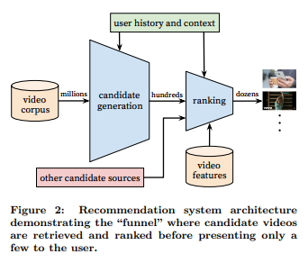
Millions to Hundreds (Candidate Generation)
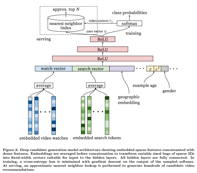
It’s a multiclass classification problem.
\[P(w_t = i|U, C) = \frac{e^{v_iu}}{\sum_{j \in V}{e^{v_ju}}}\]where \(u \in R^N\) represents an embedding of the user, context pair and \(v_j \in R^N\) represent embeddings of videos. The task of the neural network is to learn the user embeddings \(u\) as a function of the user’s history and context.
One problem with extreme multiclass classification in neural networks is the inefficient backpropagation. If the forward and backward passes are computed for over the entire corpus of millions of videos for every true label, it would be terribly inefficient. A similar problem arises in the word2vec model. Some tricks to make this efficient include Hierarchical Softmax and Negative Sampling (This blog post by Sebastian Ruder has an excellent comparison between various approaches).
A key advantage of using deep neural networks as generalization of matrix factorization is that arbitrary continuous and categorical features can be easily added to the model. Search history as well as watch history are used as features in this model. In both cases, the embeddings are averaged before being fed into the network. The user’s geographic region and the device type are embedded and concatenated. Simple binary and continuous features su as the user’s gender, logged-in state and age are input directly into the network as real values normalized to [0, 1].
Additonal notes:
- Including the watch times from the sources other than the youtube recommendations (e.g. videos embedded into various webpages) helps reduce the exploitation problem.
- Fixing the number of examples per user helps improve the live performance. It prevents a small cohort of highly active users from dominating the loss.
- Sometimes withholding the information from the classifier helps. For example, after a user searches for “Taylor Swift”, if the next homepage recommendations show the same results as the search query, they perform remarkably poorly. If the sequence information is held out from the classifier, the model does not weigh the last search heavily.
Hundreds to Dozens (Ranking)
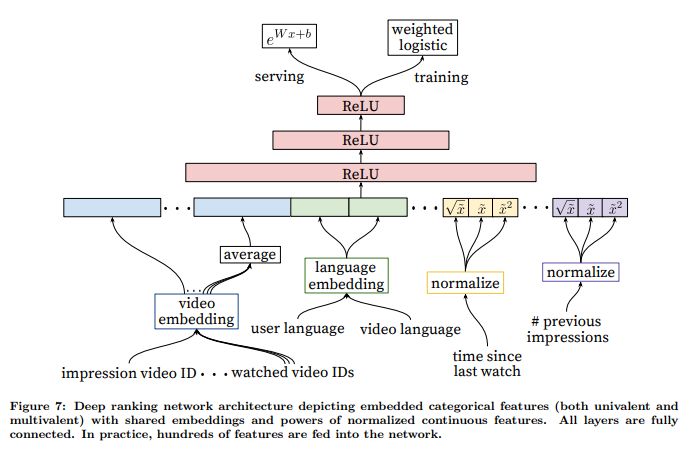
Ranking model is similar to the candidate generation model. Since there are only hundreds of videos at this stage, the model is given access to a rich set of features describing the videos and the user context pair.
Features fall into 2 main categories:
- Categorical Features - Embeddings are used to map the sparse categories to dense representations. Out-of-vocabulary values are simply mapped to 0. Categorical features can be either univalent (single value) or multivalent (multiple values). In case of a multivalent feature like the last \(N\) video IDs, the average of the embeddings is fed into the network. Categorical features in the same ID space also share underlying embeddings. For example, there exists a single global embedding of video IDs that many distinct features use - video ID of the impression, last video ID watch by the user etc.
- Continuous Features - Continuous features are normalized before being used. Along with raw normalized feature \(\widetilde{x}\), they also feed powers \(\widetilde{x}^2\) and \(\sqrt{\widetilde{x}}\) to the network. The found this to be useful for offline accuracy.
Since the goal is to predict expected watch time, each positive impression (video impression was clicked) is weighted by the observed watch time on the video. This weighted impressions are then learned by weighted logistic regression. For inference, they simply use the exponential function \(e^x\) to obtain the probabilities.
Details of the model are shown in the following image.
They experimented with various hidden layer structures and found depth to be helpful. The following table describes some results on various hidden layer configurations. Increasing the width as well as the depth seem to help increase the accuracy.
| Hidden Layers | weighted, per-user loss |
|---|---|
| None | 41.6% |
| 256 ReLU | 36.9% |
| 512 ReLU | 36.7% |
| 1024 ReLU | 35.8% |
| 512 ReLU -> 256 ReLU | 35.2% |
| 1024 ReLU -> 512 ReLU | 34.7% |
| 1024 ReLU -> 512 ReLU -> 256 ReLU | 34.6% |