Probability Primer
- Discrete Random Variables (RV) and Probability Mass Function (PMF)
- Continuous Random Variables and Probability Density Functions (PDF)
- Other probability concepts
- Bayes’ Rule
- Resources
Discrete Random Variables (RV) and Probability Mass Function (PMF)
Probability Mass Function(PMF) \(P\) maps a state of a random variable to the probability of that random variable taking on that state.
- Domain of \(P\) is the set of all possible events: \(\Omega\)
- Probabilities range from 0 to 1. \(\forall{x}\in\mathbf{x}, 0 \le P(x) \le 1\)
- Probabilities sum up to 1. \(\sum_{x \in \mathbf{x}}P(x) = 1\)
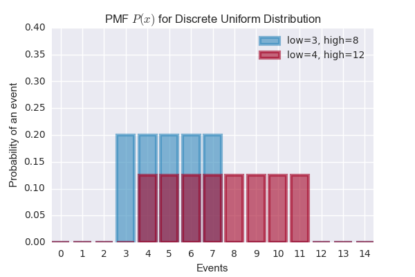
Discrete Uniform Distribution
\[P(\mathbf{x}=x_i) = \frac{1}{k}\]import matplotlib.pyplot as plt
import numpy as np
import scipy.stats as stats
import seaborn as sns
sns.set()
# Discrete Uniform distributions
uniform1 = stats.randint(low=3, high=8)
uniform2 = stats.randint(low=4, high=12)
# Plot the PMF function
a = np.arange(15)
plt.xticks(a + 0.4, a)
plt.bar(a, uniform1.pmf(a), color='#348ABD', edgecolor='#348ABD', alpha=0.60, lw='3', label='low=3, high=8')
plt.bar(a, uniform2.pmf(a), color='#A60628', edgecolor='#A60628', alpha=0.60, lw='3', label='low=4, high=12')
plt.ylim(0, 0.4)
plt.xlabel('Events')
plt.ylabel('Probability of an event')
plt.title('PMF $P(x)$ for Discrete Uniform Distribution')
plt.legend()
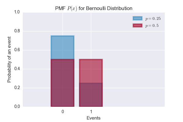
Bernoulli Distribution
\[P(x) = \begin{cases} 1-p, & \text{if $k=0$} \\ p, & \text{if $k=1$} \end{cases}\]\(p\) is the parameter of the distribution. Expected value of the distribution is \(p\).
import matplotlib.pyplot as plt
import numpy as np
import scipy.stats as stats
import seaborn as sns
sns.set()

# Bernoulli distributions
bernoulli1 = stats.bernoulli(p=0.25)
bernoulli2 = stats.bernoulli(p=0.5)

# Plot the PMF function
a = np.arange(2)
plt.xticks(a + 0.4, a)
plt.bar(a, bernoulli1.pmf(a), color='#348ABD', edgecolor='#348ABD', alpha=0.60, lw='3', label='$p=0.25$')
plt.bar(a, bernoulli2.pmf(a), color='#A60628', edgecolor='#A60628', alpha=0.60, lw='3', label='$p=0.5$')
plt.xlim(-1, 4)
plt.ylim(0, 1)
plt.xlabel('Events')
plt.ylabel('Probability of an event')
plt.title('PMF $P(x)$ for Bernoulli Distribution')
plt.legend()
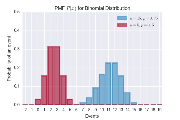
Binomial Distribution
A binomial distribution is parameterized by \(n\) and \(p\). It models the number of successes in a sequence of \(n\) independent experiments, each with success probability \(p\). For \(n=1\), the binomial distribution is a Bernoulli distribution.
\[P(\mathbf{x} = k) = {n \choose k}p^kq^{n-k}, \text{where } k \in \{0, 1, 2,..n\}\]import matplotlib.pyplot as plt
import numpy as np
import scipy.stats as stats
import seaborn as sns
sns.set()
# Binomial distributions
binomial1 = stats.binom(15, 0.75)
binomial2 = stats.binom(5, 0.5)
# Plot the PMF function
a = np.arange(-2, 20)
plt.xticks(a + 0.4, a)
plt.bar(a, binomial1.pmf(a), color='#348ABD', edgecolor='#348ABD', alpha=0.60, lw='3', label='$n=15, p=0.75$')
plt.bar(a, binomial2.pmf(a), color='#A60628', edgecolor='#A60628', alpha=0.60, lw='3', label='$n=5, p=0.5$')
plt.ylim(0, 0.5)
plt.xlabel('Events')
plt.ylabel('Probability of an event')
plt.title('PMF $P(x)$ for Binomial Distribution')
plt.legend()
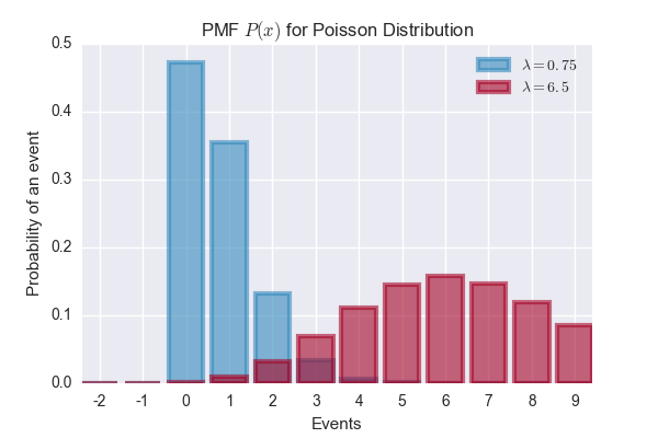
Poisson Distribution
Random Variable \(\mathbf{z}\) is Poisson-distributed if:
\[P(\mathbf{z}=k) = \frac{\lambda^k e^{-\lambda}}{k!}, k = 0, 1, 2,...\]\(\lambda\) is the parameter of the distribution - it can be any positive number. Expected value of the distribution \(\mathbf{z}\) is:
\[E[\mathbf{z}] = \lambda\]import matplotlib.pyplot as plt
import numpy as np
import scipy.stats as stats
import seaborn as sns
sns.set()
# Poisson distributions
poisson1 = stats.poisson(0.75)
poisson2 = stats.poisson(6.5)
# Plot the PMF function
a = np.arange(-2, 10)
plt.xticks(a + 0.4, a)
plt.bar(a, poisson1.pmf(a), color='#348ABD', edgecolor='#348ABD', alpha=0.60, lw='3', label='$\lambda=0.75$')
plt.bar(a, poisson2.pmf(a), color='#A60628', edgecolor='#A60628', alpha=0.60, lw='3', label='$\lambda=6.5$')
plt.ylim(0, 0.5)
plt.xlabel('Events')
plt.ylabel('Probability of an event')
plt.title('PMF $P(x)$ for Poisson Distribution')
plt.legend()
Continuous Random Variables and Probability Density Functions (PDF)
We describe continuous random variables using Probabiliy Density Function(PDF) \(p\) instead of probability mass function.
- It’s important to note that \(p(x)\) is not probability. \(p(x)\) is the probability density.
- Densities are positive. \(\forall{x}\in\mathbf{x}, p(x) \ge 0\)
- \(p(x)\delta{x}\) represents the probability of landing inside \(\delta{x}\) sized region. Since \(p(x)\delta{x}\) is the probability, it should integrate to 1. \(\int p(x)dx = 1\)
- Example: If a random variable \(\mathbf{x}\) is represented by the uniform distribution that takes values from real value \(a\) to real value \(b\), it can be represented as \(\mathbf{x} \sim U(a, b)\).
Uniform Distribution
\[p(x) = \frac{1}{b - a}\]Exponential Distribution
\[p(x) = e^{-x}, \text{where } x >= 0\]Normal Distribution
\[p(x) = \frac{e^{-x^2/2}}{\sqrt{2\pi}}\]Other probability concepts
Marginal Probability
Sometimes we know the probability distribution over a set of variables and we want to know the probability distribution over just a subset of them. The probability distribution over the subset is known as the marginal probability distribution.
\[p(x) = \int p(x, y)dy\]Considitional Probability
In many cases, we are interested in the probability of some event, given that some other event has happened. This is called a conditional probability.
\[P(\mathbf{y} = y | \mathbf{x} = x) = \frac{P(\mathbf{y} = y, \mathbf{x} = x)}{P(\mathbf{x} = x)}\]Chain Rule of Probabilities
\[P(a,b,c) = P(a|b,c)P(b|c)P(c)\]Independence and Conditional Independence
Two random variables \(\mathbf{x}\) and \(\mathbf{y}\) are independent if their probability distribution can be expressed as a product of two factors.
\[\forall x\in\textbf{x},y\in\textbf{y}, p(\textbf{x}=x, \textbf{y}=y) = p(\textbf{x}=x)p(\textbf{y}=y)\]Expectation, Variance and Covariance
Expected value of a function \(f(x)\) over the random variable \(\textbf{x}\) is defined as:
\[E_{x \sim p}[f(x)] = \int p(x)f(x)dx\]Bayes’ Rule
\[P(x|y) = \frac{P(x)P(y|x)}{P(y)}\]Resources
- Probability Cheatsheet
- Probability and Information Theory chapter in the Deep Learning book.
- Introduction to Probability and Statistics course from MIT OpenCourseWare.